
Tracé de courbes
Contenu
Tracé de courbes#
Pour tracer des courbes, Python n’est pas suffisant et nous avons besoin de la bibliothèque Matplotlib utilisée dans ce cours. Si vous ne disposez pas de cette bibliothèque, vous pouvez consulter la page Introduction à Python pour installer l’environnement adapté.
Dans cette page, nous présentons deux styles de programmation :
le style « pyplot » qui utilise directement des fonctions du module
pyplot;le style « Oriénté Objet (OO) » qui est recommandé dans la documentation de Matplotlib.
Note
Vous pouvez trouver sur internet d’anciens exemples qui utilisent l’interface pylab via from pylab import *. Cette approche est à présent obsolète et fortement déconseillée par la documentation de Matplotlib.
Quel que soit le style de programmation, il est nécessaire d’importer le module pyplot de matplotlib. On lui donne en général l’alias plt. On précise ensuite ce module lors de l’appel des fonctions (voir les exemples ci-dessous). Pour en savoir plus sur la notion d’importation, vous pouvez consulter la page Modules et importations.
Création d’une courbe#
Utilisation de plot()#
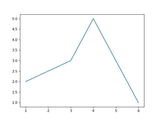
L’instruction plot() permet de tracer des courbes qui relient des points dont les abscisses et ordonnées sont fournies en arguments.
Exemple 1
Style « pyplot »
import numpy as np
import matplotlib.pyplot as plt

plt.plot([1, 3, 4, 6], [2, 3, 5, 1])

plt.show() # affiche la figure à l'écran
Style « Orienté Objet »
import numpy as np
import matplotlib.pyplot as plt

fig, ax = plt.subplots()
ax.plot([1, 3, 4, 6], [2, 3, 5, 1])

plt.show() # affiche la figure à l'écran
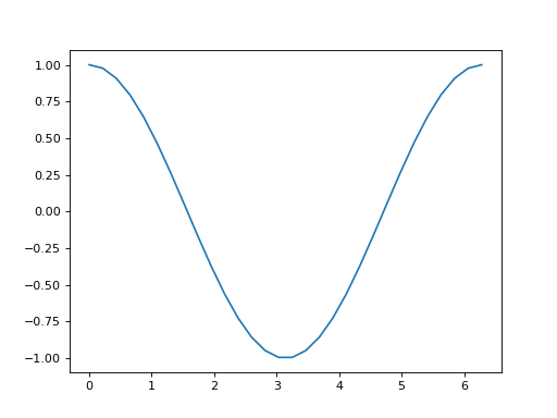
Exemple 2
Dans cet exemple, nous allons tracer la fonction cosinus.
Style « pyplot »
import numpy as np
import matplotlib.pyplot as plt

x = np.linspace(0, 2*np.pi, 30)
y = np.cos(x)

plt.plot(x, y)

plt.show() # affiche la figure à l'écran
Style « Orienté Objet »
import numpy as np
import matplotlib.pyplot as plt

x = np.linspace(0, 2*np.pi, 30)
y = np.cos(x)

fig, ax = plt.subplots()
ax.plot(x, y)

plt.show() # affiche la figure à l'écran
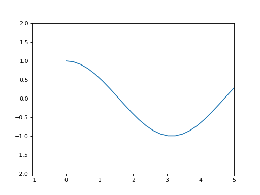
Définition du domaine des axes - xlim(), ylim() et axis()#
Dans le style pyplot, il est possible fixer les domaines des abscisses et des ordonnées en utilisant les fonctions xlim(), ylim() ou axis().
xlim(xmin, xmax)
ylim(ymin, ymax)
axis() permet de fixer simultanément les domaines des abscisses et des ordonnées.
Note
Avec axis(), les limites du domaine doivent être données dans une liste où les valeurs sont entourées par des crochets [ et ].
axis([xmin, xmax, ymin, ymax])
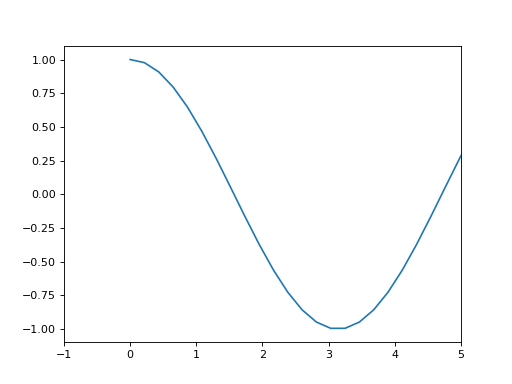
Exemple avec xlim()
Avertissement
Dans le style « Orienté Objet », il faut utiliser set_xlim().
Style « pyplot »
import numpy as np
import matplotlib.pyplot as plt

x = np.linspace(0, 2*np.pi, 30)
y = np.cos(x)

plt.plot(x, y)
plt.xlim(-1, 5)

plt.show()
Style « Orienté Objet »
import numpy as np
import matplotlib.pyplot as plt

x = np.linspace(0, 2*np.pi, 30)
y = np.cos(x)

fig, ax = plt.subplots()
ax.plot(x, y)
ax.set_xlim(-1, 5)

plt.show()
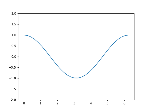
Exemple avec ylim()
Avertissement
Dans le style « Orienté Objet », il faut utiliser set_ylim().
Style « pyplot »
import numpy as np
import matplotlib.pyplot as plt

x = np.linspace(0, 2*np.pi, 30)
y = np.cos(x)

plt.plot(x, y)
plt.ylim(-2, 2)

plt.show()
Style « Orienté Objet »
import numpy as np
import matplotlib.pyplot as plt

x = np.linspace(0, 2*np.pi, 30)
y = np.cos(x)

fig, ax = plt.subplots()
ax.plot(x, y)
ax.set_ylim(-2, 2)

plt.show()
Exemple avec axis()
Style « pyplot »
import numpy as np
import matplotlib.pyplot as plt

x = np.linspace(0, 2*np.pi, 30)
y = np.cos(x)

plt.plot(x, y)
plt.axis([-1, 5, -2, 2])

plt.show()
Style « Orienté Objet »
import numpy as np
import matplotlib.pyplot as plt

x = np.linspace(0, 2*np.pi, 30)
y = np.cos(x)

fig, ax = plt.subplots()
ax.plot(x, y)
ax.axis([-1, 5, -2, 2])

plt.show()
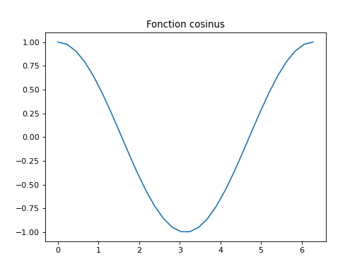
Ajout d’un titre - title()#
Dans le style pyplot, on peut ajouter un titre grâce à l’instruction title().
Style « pyplot »
import numpy as np
import matplotlib.pyplot as plt

x = np.linspace(0, 2*np.pi, 30)
y = np.cos(x)

plt.plot(x, y)
plt.title("Fonction cosinus")

plt.show()
Style « Orienté Objet »
Avertissement
Dans le style « Orienté Objet », il faut utiliser set_title().
import numpy as np
import matplotlib.pyplot as plt

x = np.linspace(0, 2*np.pi, 30)
y = np.cos(x)

fig, ax = plt.subplots()
ax.plot(x, y)
ax.set_title("Fonction cosinus")

plt.show()
Ajout d’une légende - legend()#
Style « pyplot »
import numpy as np
import matplotlib.pyplot as plt

x = np.linspace(0, 2*np.pi, 30)
y = np.cos(x)

plt.plot(x, y, label="cos(x)")
plt.legend()

plt.show()
Style « Orienté Objet »
import numpy as np
import matplotlib.pyplot as plt

x = np.linspace(0, 2*np.pi, 30)
y = np.cos(x)

fig, ax = plt.subplots()
ax.plot(x, y, label="cos(x)")
ax.legend()

plt.show()
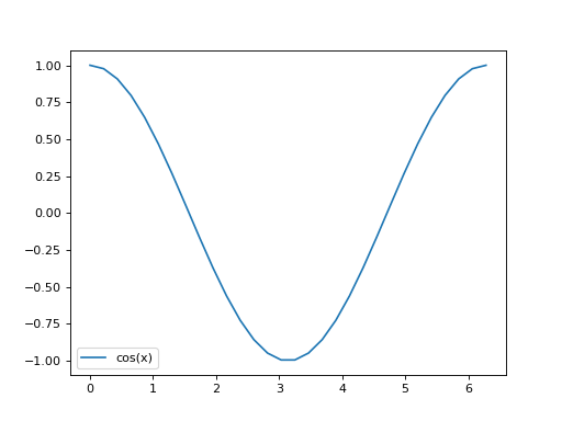
Avertissement
Pour faire afficher le label, il ne faut pas oublier de faire appel à l’instruction legend().
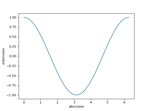
Labels sur les axes - xlabel() et ylabel()#
Dans le style pyplot, des labels sur les axes peuvent être ajoutés avec les fonctions xlabel() et ylabel().
Style « pyplot »
import numpy as np
import matplotlib.pyplot as plt

x = np.linspace(0, 2*np.pi, 30)
y = np.cos(x)

plt.plot(x, y)
plt.xlabel("abscisses")
plt.ylabel("ordonnées")

plt.show()
Style « Orienté Objet »
Avertissement
Dans le style « Orienté Objet », il faut utiliser set_xlabel() et set_ylabel().
import numpy as np
import matplotlib.pyplot as plt

x = np.linspace(0, 2*np.pi, 30)
y = np.cos(x)

fig, ax = plt.subplots()
ax.plot(x, y)
ax.set_xlabel("abscisses")
ax.set_ylabel("ordonnées")

plt.show()
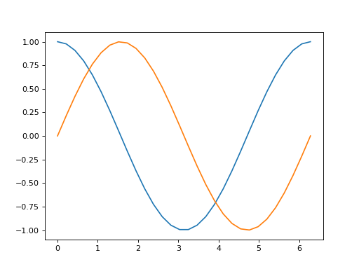
Affichage de plusieurs courbes#
Pour afficher plusieurs courbes sur un même graphe, on peut procéder de la façon suivante :
Style « pyplot »
import numpy as np
import matplotlib.pyplot as plt

x = np.linspace(0, 2*np.pi, 30)
y1 = np.cos(x)
y2 = np.sin(x)

plt.plot(x, y1)
plt.plot(x, y2)

plt.show()
Style « Orienté Objet »
import numpy as np
import matplotlib.pyplot as plt

x = np.linspace(0, 2*np.pi, 30)
y1 = np.cos(x)
y2 = np.sin(x)

fig, ax = plt.subplots()
ax.plot(x, y1)
ax.plot(x, y2)

plt.show()
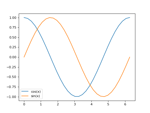
Exemple avec un légende#
Style « pyplot »
import numpy as np
import matplotlib.pyplot as plt

x = np.linspace(0, 2*np.pi, 30)
y1 = np.cos(x)
y2 = np.sin(x)

plt.plot(x, y1, label="cos(x)")
plt.plot(x, y2, label="sin(x)")
plt.legend()

plt.show()
Style « Orienté Objet »
import numpy as np
import matplotlib.pyplot as plt

x = np.linspace(0, 2*np.pi, 30)
y1 = np.cos(x)
y2 = np.sin(x)

fig, ax = plt.subplots()
ax.plot(x, y1, label="cos(x)")
ax.plot(x, y2, label="sin(x)")
ax.legend()

plt.show()
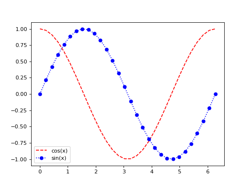
Formats de courbes#
Il est possible de préciser la couleur, le style de ligne et de symbole (« marker ») en ajoutant une chaîne de caractères de la façon suivante :
import numpy as np
import matplotlib.pyplot as plt

x = np.linspace(0, 2*np.pi, 30)
y1 = np.cos(x)
y2 = np.sin(x)

plt.plot(x, y1, "r--", label="cos(x)")
plt.plot(x, y2, "b:o", label="sin(x)")
plt.legend()

plt.show()
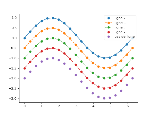
Style de ligne#
Les chaînes de caractères suivantes permettent de définir le style de ligne :
Chaîne |
Effet |
|---|---|
|
ligne continue |
|
tirets |
|
ligne en pointillé |
|
tirets points |
Avertissement
Si on ne veut pas faire apparaître de ligne, il suffit d’indiquer un symbole sans préciser un style de ligne.
Exemple
import numpy as np
import matplotlib.pyplot as plt

x = np.linspace(0, 2*np.pi, 20)
y = np.sin(x)

plt.plot(x, y, "o-", label="ligne -")
plt.plot(x, y-0.5, "o--", label="ligne --")
plt.plot(x, y-1, "o:", label="ligne :")
plt.plot(x, y-1.5, "o-.", label="ligne -.")
plt.plot(x, y-2, "o", label="pas de ligne")
plt.legend()

plt.show()
Symbole (« marker »)#
Les chaînes de caractères suivantes permettent de définir le symbole (« marker ») :
Chaîne |
Effet |
|---|---|
|
point marker |
|
pixel marker |
|
circle marker |
|
triangle_down marker |
|
triangle_up marker |
|
triangle_left marker |
|
triangle_right marker |
|
tri_down marker |
|
tri_up marker |
|
tri_left marker |
|
tri_right marker |
|
square marker |
|
pentagon marker |
|
star marker |
|
hexagon1 marker |
|
hexagon2 marker |
|
plus marker |
|
x marker |
|
diamond marker |
|
thin_diamond marker |
|
vline marker |
|
hline marker |
Couleur#
Les chaînes de caractères suivantes permettent de définir la couleur :
Chaîne |
Couleur en anglais |
Couleur en français |
|---|---|---|
|
blue |
bleu |
|
green |
vert |
|
red |
rouge |
|
cyan |
cyan |
|
magenta |
magenta |
|
yellow |
jaune |
|
black |
noir |
|
white |
blanc |
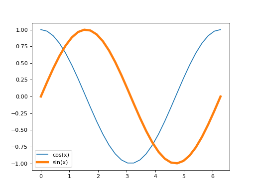
Largeur de ligne#
Pour modifier la largeur des lignes, il est possible de changer la valeur de l’argument linewidth.
import numpy as np
import matplotlib.pyplot as plt

x = np.linspace(0, 2*np.pi, 30)
y1 = np.cos(x)
y2 = np.sin(x)

plt.plot(x, y1, label="cos(x)")
plt.plot(x, y2, label="sin(x)", linewidth=4)
plt.legend()

plt.show()
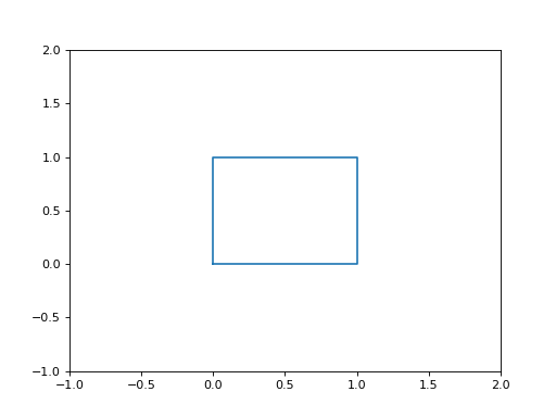
Tracé de formes#
Comme la fonction plot() ne fait que relier des points, il est possible de lui fournir plusieurs points avec la même abscisse.
Style « pyplot »
import numpy as np
import matplotlib.pyplot as plt

x = np.array([0, 1, 1, 0, 0])
y = np.array([0, 0, 1, 1, 0])

plt.plot(x, y)
plt.xlim(-1, 2)
plt.ylim(-1, 2)

plt.show()
Style « Orienté Objet »
import numpy as np
import matplotlib.pyplot as plt

x = np.array([0, 1, 1, 0, 0])
y = np.array([0, 0, 1, 1, 0])

fig, ax = plt.subplots()
ax.plot(x, y)
ax.set_xlim(-1, 2)
ax.set_ylim(-1, 2)

plt.show()
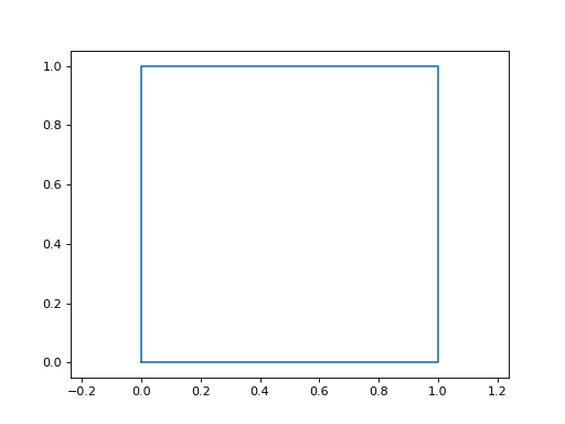
L’instruction axis("equal")#
L’instruction axis("equal") permet d’avoir la même échelle sur l’axe des abscisses et l’axe des ordonnées afin de préserver la forme lors de l’affichage. En particulier, grâce à cette commande un carré apparaît vraiment comme un carré, de même pour un cercle.
Style « pyplot »
import numpy as np
import matplotlib.pyplot as plt

x = np.array([0, 1, 1, 0, 0])
y = np.array([0, 0, 1, 1, 0])

plt.plot(x, y)
plt.axis("equal")

plt.show()
Style « Orienté Objet »
import numpy as np
import matplotlib.pyplot as plt

x = np.array([0, 1, 1, 0, 0])
y = np.array([0, 0, 1, 1, 0])

fig, ax = plt.subplots()
ax.plot(x, y)
ax.axis("equal")

plt.show()
Il est aussi possible de fixer le domaine des abscisses en utilisant axis().
Style « pyplot »
import numpy as np
import matplotlib.pyplot as plt

x = np.array([0, 1, 1, 0, 0])
y = np.array([0, 0, 1, 1, 0])

plt.plot(x, y)
plt.axis("equal")
plt.axis([-1, 2, -1, 2])

plt.show()
Style « Orienté Objet »
import numpy as np
import matplotlib.pyplot as plt

x = np.array([0, 1, 1, 0, 0])
y = np.array([0, 0, 1, 1, 0])

fig, ax = plt.subplots()
ax.plot(x, y)
ax.axis("equal")
ax.axis([-1, 2, -1, 2])

plt.show()
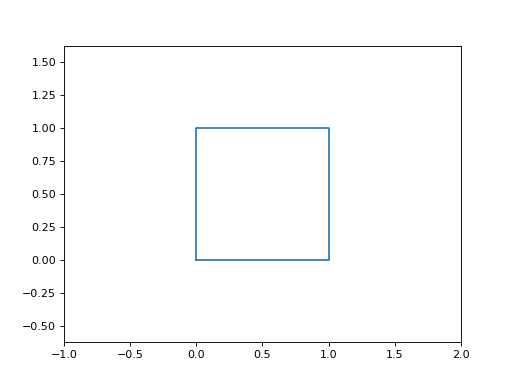
Note
On peut noter que les limites ne sont pas respectées en même temps pour les abscisses et les ordonnées, mais la forme est bien préservée.
Tracé d’un cercle#
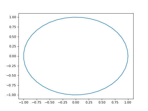
On peut tracer utiliser une courbe paramétrique pour tracer un cercle.
Sans axis("equal"), la courbe n’apparaît pas comme un cercle.
Style « pyplot »
import numpy as np
import matplotlib.pyplot as plt

theta = np.linspace(0, 2*np.pi, 40)

x = np.cos(theta)
y = np.sin(theta)

plt.plot(x, y)

plt.show()
Style « Orienté Objet »
import numpy as np
import matplotlib.pyplot as plt

theta = np.linspace(0, 2*np.pi, 40)

x = np.cos(theta)
y = np.sin(theta)

fig, ax = plt.subplots()
ax.plot(x, y)

plt.show()
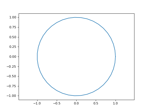
Avec axis("equal"), on obtient bien un cercle.
Style « pyplot »
import numpy as np
import matplotlib.pyplot as plt

theta = np.linspace(0, 2*np.pi, 40)

x = np.cos(theta)
y = np.sin(theta)

plt.plot(x, y)
plt.axis("equal")

plt.show()
Style « Orienté Objet »
import numpy as np
import matplotlib.pyplot as plt

theta = np.linspace(0, 2*np.pi, 40)

x = np.cos(theta)
y = np.sin(theta)

fig, ax = plt.subplots()
ax.plot(x, y)
ax.axis("equal")

plt.show()
Il est aussi possible de fixer le domaine des abscisses en utilisant axis().
Style « pyplot »
import numpy as np
import matplotlib.pyplot as plt

theta = np.linspace(0, 2*np.pi, 40)

x = np.cos(theta)
y = np.sin(theta)

plt.plot(x, y)
plt.axis("equal")
plt.axis([-3, 3, -3, 3])

plt.show()
Style « Orienté Objet »
import numpy as np
import matplotlib.pyplot as plt

theta = np.linspace(0, 2*np.pi, 40)

x = np.cos(theta)
y = np.sin(theta)

fig, ax = plt.subplots()
ax.plot(x, y)
ax.axis("equal")
ax.axis([-3, 3, -3, 3])

plt.show()
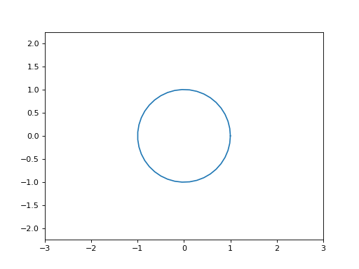
Note
A nouveau, on peut noter que les limites ne sont pas respectées en même temps pour les abscisses et les ordonnées, mais la forme est bien préservée.
Voir aussi
La documentation de Matplotlib (en anglais) : https://matplotlib.org/
Le tutoriel de pyplot sur le site Matplotlib (en anglais) : https://matplotlib.org/stable/tutorials/introductory/pyplot.html
Le tutoriel Matplotlib de Nicolas P. Rougier (en anglais) : https://github.com/rougier/matplotlib-tutorial
Le livre « Scientific Visualization: Python + Matplotlib » de Nicolas P. Rougier (en anglais) : https://github.com/rougier/scientific-visualization-book